Linear Regression¶

This tutorial guides you through building and training a linear regression model with Taktiny.

You will learn how to:

Construct a linear model using taktiny.nn.Linear.
Generate synthetic data and batch it with taktiny.data.DataLoader.
Train the model using taktiny.trainer.Trainer with Mean Squared Error (MSE).
Inspect learned parameters (kernel and bias).

1. Install Taktiny¶

If Taktiny isn’t installed in your Python environment, you can install Taktiny from GitHub by using either pip or uv

uv add -U git+https://github.com/solitariusai/taktiny.git@experiment
# or
# pip install -U git+https://github.com/solitariusai/taktiny.git@experiment

2. Import Packages¶

import jax
import jax.numpy as jnp
import matplotlib.pyplot as plt

from taktiny import nn
from taktiny.data import Batch, DataLoader, train_validation_split
from taktiny.trainer import DatasetConfig, Trainer, TrainingConfig

3. Define the Regression Model¶

In Taktiny, models inherit from taktiny.nn.Module. Every weight is a taktiny.nn.Parameter registered as a JAX PyTree leaf.

class LinearRegression(nn.Module):
    def __init__(self, in_features: int, out_features: int = 1, *, rngs: nn.Rngs):
        self.linear = nn.Linear(in_features, out_features, rngs=rngs)

    def __call__(self, x: jax.Array) -> jax.Array:
        return self.linear(x)

# Initialize with a seeded PRNG state
rngs = nn.Rngs(42)
model = LinearRegression(in_features=3, out_features=1, rngs=rngs)

4. Generating Synthetic Data¶

We generate synthetic points with a known linear relation: \(y = X w + b + \epsilon\). Note that rngs is callable and returns a new PRNG key on each call, so you can continue using rngs() after model initialization.

# Ground-truth weights and bias
true_w = jnp.array([[1.5], [-2.0], [0.5]])
true_b = 0.8

# Generate 200 random points in R^3
n_samples = 200
xs = jax.random.normal(rngs(), (n_samples, 3))
noise = 0.05 * jax.random.normal(rngs(), (n_samples, 1))
ys = xs @ true_w + true_b + noise

# Package as a list of records
dataset = [{"x": xs[i], "y": ys[i]} for i in range(n_samples)]

# Train-validation split
train_data, val_data = train_validation_split(dataset, validation_size=0.2, seed=42)

# Build DataLoaders
train_loader = DataLoader(train_data, operations=[Batch(batch_size=16)])
val_loader = DataLoader(val_data, operations=[Batch(batch_size=16)])

5. Training with `Trainer`¶

Define Mean Squared Error Loss¶

The loss function receives the model instance and batch dictionary:

def mse_loss(m: LinearRegression, batch: dict[str, jax.Array]) -> jax.Array:
    predictions = m(batch["x"])
    targets = batch["y"]
    return jnp.mean((predictions - targets) ** 2)

Configure and Run the Trainer¶

training_config = TrainingConfig(
    max_steps=100,
    learning_rate=0.05,
    log_interval=10,
    eval_strategy="steps",
    eval_steps=25,
)

dataset_config = DatasetConfig(
    train_dataloader=train_loader,
    validation_dataloader=val_loader,
)

trainer = Trainer(
    model=model,
    training_config=training_config,
    dataset_config=dataset_config,
    loss_fn=mse_loss,
)

trainer.train()

6. Inspect Learned Parameters¶

After training, access the learned parameters directly:

print("True kernel:    [1.5, -2.0, 0.5]")
print("Learned kernel:", model.linear.kernel.value.squeeze())
print("True bias:      0.8")
print("Learned bias:  ", float(model.linear.bias.value.squeeze()))

7. Functional Inference¶

You can use jax.jit directly to the model instance for compiled inference:

sample = jnp.array([[1.0, 1.0, 1.0]])
jit_model = jax.jit(model)
pred = jit_model(sample)
print("Prediction for [1, 1, 1]:", float(pred[0, 0]))

8. Visualization¶

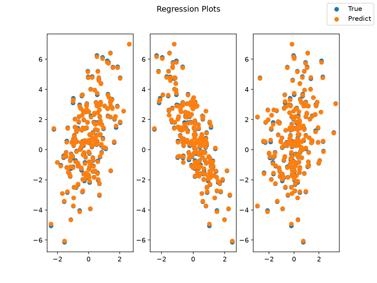
Plot the target and model predictions against each input feature using matplotlib.

fig, axs = plt.subplots(1, 3, figsize=(8, 6))

pred = jit_model(xs)

for i in range(3):
    axs[i].scatter(xs[:, i], ys.squeeze(), label='True')
    axs[i].scatter(xs[:, i], pred.squeeze(), label='Predict')

fig.legend(*axs[0].get_legend_handles_labels())
fig.suptitle("Regression Plots")

plt.show()

You should see something like this.